The science behind Two-Level Systems

The ingredients to understand the two-level system [1][2] require a few concepts.
The following sections will introduce the and develop these concepts and at the end, we will summarize what we have learned.

First, we will examine the states of our system. Then, we will see how these states can indeed be thought of as vectors on the Bloch sphere and why this is particularly useful. Finally, we will see how we control the dynamics of the system, i.e. how the vectors are rotated around on the sphere as time passes.

The states

In this application, the two-level system consists of two internal electronic energy levels of an atom that can be controlled by a laser.

We can label the energy levels according to their energies

These states can also form a general superposition state

Here a and b are complex numbers and their square modulus give the probability of being in the corresponding state

These probabilities must add to 1!

Any choice of a and b that satisfies this condition represents a physical state of our system.

The Bloch Sphere

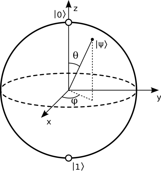
A fantastic feature of the two-level system is the ability to express the states as geometrical vectors on a sphere of radius 1, known as the Bloch sphere.
To completely specify the vectors, we need to define the following angles

Every combination of the two angles now uniquely describe a vector of length 1 on the Bloch sphere. Neat!

We would like this geometrical description to carry some physical meaning. To this end, we write the general superposition state as

Note that this simply means we have chosen

So what are now the probabilities of being in either of the two states? We can just put it into the previous definition to calculate it

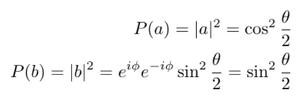
Is this consistent with our probability conditions? Yes, it is!

for any choice of angles. Note that the angle does not enter at all in this expression. Only the angle θ determine how the probabilities are distributed. Speaking of, we are now ready to see why this was a particularly smart way of writing our states. Let us put in the boundary values θ=0 and θ=π :

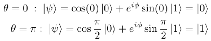
We are now ready to harvest the first fruits of our labor:

1. When θ=0 the vector points directly ‘up’ and the system is in the ground state with probability 1.
2. When θ=π the vector points directly ‘down’ and the system is in the excited state with probability 1.
3. When the angle is anywhere in between, the system is in a superposition state with probabilities given by our earlier calculations. The more the vector points up (down) the larger is the probability of being in the ground state (excited state).

In fact these three statements can be combined and we arrive at the following geometric interpretation:
Our states are vectors on a sphere with radius 1.
The ‘amount’ the vector points along the z-axis gives the probabilities in our system

This statement along with the interpretation of our ground state and excited state summarizes our entire discussion up until now.

Dynamics - Rotating States on the Bloch Sphere

From the previous section. we know how to describe the states as vectors on the Bloch sphere. But what if we interacted with the system somehow? What would happen to the system? How do we describe the dynamics? To answer this question we put another cornerstone of quantum mechanics into action: the Schrödinger equation (SE)

Let us dissect the equation in its components. From the previous sections, we recognize the state vector which we found could be written as

On the left-hand side of the SE, we have the derivative of the state with respect to time. That is nice because our goal is to examine how the system evolves as time goes on. We also have the complex unit ‘i’ on the left-hand side. Without getting too technical, this is necessary for quantum mechanics to exhibit wave-like nature (iIf it was not there, the Universe would be dead and decayed).

On the right-hand side, we again have the state, this time is multiplied by the Hamiltonian ‘H’. The Hamiltonian is the centerpiece in describing the time evolution and through this object, we can control the system. The Hamiltonian for our two-level system can be written

where σx and σz are so-called Pauli spin matrices and is the so-called Rabi frequency and detuning respectively. It is only at this point where we have used anything related to our specific problem of controlling atoms with light! Loosely speaking, shows us how intense the light is and tells us how closely the wavelength of the light matches the energy difference between the two levels. Note that both quantities can both be negative and change in time.

The final idea, that ties this section to the previous one, is that the Pauli spin matrices are so-called generators of rotations!
σx (σz) is responsible for rotating our vector around the x-axis (z-axis), the size of () determines how fast the vector rotates, and the sign of ()determines if the rotation is clockwise or counterclockwise.

Putting it all together

1. States are represented as vectors on a sphere of radius 1.
2. The angle made with the vector and the z-axis determines the probability of the ground state and the excited state.
3. Time evolution corresponds to rotating the vectors around on the sphere depending on the size and the sign of and, which are physical characteristics of the laser and the atom.

References:

[1] P. W. Milonni, J.H. Eberly (2010). Laser Physics (Ch. 9)

[2] M. A. Nielsen, I. L. Chuang (2010). Quantum Computation and Quantum Information (Ch. 1)